Visible Knowledge Mining utilizing Parallel Coordinates

Some years in the past, when working as a advisor, I used to be deriving a comparatively complicated ML algorithm, and was confronted with the problem of creating the interior workings of that algorithm clear to my stakeholders. That’s after I first got here to make use of parallel coordinates – as a result of visualizing the relationships between two, three, perhaps 4 or 5 variables is straightforward. However as quickly as you begin working with vectors of upper dimension (say, 13, for instance), the human thoughts oftentimes is unable to understand this complexity. Enter parallel coordinates: a device so easy, but so efficient, that I typically marvel why it’s so little in use in on a regular basis EDA (my groups are an exception). Therefore, on this article, I’ll share with you the advantages of parallel coordinates based mostly on the Wine Dataset, highlighting how this system may help uncover correlations, patterns, or clusters within the knowledge with out shedding the semantics of options (e.g., in PCA). 

What are Parallel Coordinates

Parallel coordinates are a typical technique of visualizing high-dimensional datasets. And sure, that’s technically right, though this definition doesn’t totally seize the effectivity and class of the strategy. In contrast to in a regular plot, the place you could have two orthogonal axes (and therefore two dimensions that you may plot), in parallel coordinates, you could have as many vertical axes as you could have dimensions in your dataset. This implies an statement could be displayed as a line that crosses all axes at its corresponding worth. Need to be taught a flowery phrase to impress on the subsequent hackathon? “Polyline”, that’s the right time period for it. And patterns then seem as bundles of polylines with related behaviour. Or, extra particularly: clusters seem as bundles, whereas correlations seem as trajectories with constant slopes throughout adjoining axes. 

Marvel why not simply do PCA (Principal Part Evaluation)? In parallel coordinates, we retain all the unique options, that means we don’t condense the knowledge and challenge it right into a lower-dimensional area. So this eases interpretation loads, each for you and on your stakeholders! However (sure, over all the joy, there should nonetheless be a however…) you need to take excellent care to not fall into the overplotting-trap. When you don’t put together the info rigorously, your parallel coordinates simply grow to be unreadable – I’ll present you within the walkthrough that function choice, scaling, and transparency changes could be of nice assist.

Btw. I ought to point out Prof. Alfred Inselberg right here. I had the honour to dine with him in 2018 in Berlin. He’s the one who acquired me hooked on parallel coordinates. And he’s additionally the godfather of parallel coordinates, proving their worth in a large number of use instances within the Nineteen Eighties. 

Proving my Level with the Wine Dataset

For this demo, I selected the Wine Dataset. Why? First, I like wine. Second, I requested ChatGPT for a public dataset that’s related in construction to one among my firm’s datasets I’m at present engaged on (and I didn’t wish to tackle all the effort to publish/anonymize/… firm knowledge). Third, this dataset is well-researched in lots of ML and Analytics purposes. It comprises knowledge from the evaluation of 178 wines grown by three grape cultivars in the identical area of Italy. Every statement has 13 steady attributes (assume alcohol, flavonoid focus, proline content material, color depth,…). And the goal variable is the category of the grape.

So that you can comply with by means of, let me present you learn how to load the dataset in Python.

import pandas as pd # Load Wine dataset from UCI uci_url = "https://archive.ics.uci.edu/ml/machine-learning-databases/wine/wine.knowledge" # Outline column names based mostly on the wine.names file col_names = [     "Class", "Alcohol", "Malic_Acid", "Ash", "Alcalinity_of_Ash", "Magnesium",     "Total_Phenols", "Flavanoids", "Nonflavanoid_Phenols", "Proanthocyanins",     "Color_Intensity", "Hue", "OD280/OD315", "Proline" ] # Load the dataset df = pd.read_csv(uci_url, header=None, names=col_names) df.head()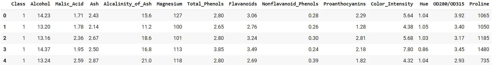

Good. Now, let’s derive a naïve plot as a baseline.

First Step: Constructed-In Pandas

Let’s use the built-in pandas plotting operate:

from pandas.plotting import parallel_coordinates import matplotlib.pyplot as plt plt.determine(figsize=(12,6)) parallel_coordinates(df, 'Class', colormap='viridis') plt.title("Parallel Coordinates Plot of Wine Dataset (Unscaled)") plt.xticks(rotation=45) plt.present()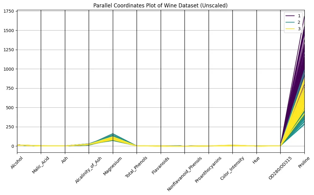

Seems good, proper? 

No, it doesn’t. You definitely are capable of discern the lessons on the plot, however the variations in scaling make it exhausting to check throughout axes. Evaluate the orders of magnitude of proline and hue, for instance: proline has a powerful optical dominance, simply due to scaling. An unscaled plot seems to be nearly meaningless, or no less than very tough to interpret. Even so, faint bundles over lessons appear to look, so let’s take this as a promise for what’s but to return…

It’s all about Scale

Lots of you (everybody?) are accustomed to the min-max scaling from ML preprocessing pipelines. So let’s not use that. I’ll do some standardization of the info, i.e., we do Z-scaling right here (every function can have a imply of zero and unit variance), to present all axes the identical weight. 

from sklearn.preprocessing import StandardScaler # Separate options and goal options = df.drop("Class", axis=1) scaler = StandardScaler() scaled = scaler.fit_transform(options) # Reconstruct a DataFrame with scaled options scaled_df = pd.DataFrame(scaled, columns=options.columns) scaled_df["Class"] = df["Class"] plt.determine(figsize=(12,6)) parallel_coordinates(scaled_df, 'Class', colormap='plasma', alpha=0.5) plt.title("Parallel Coordinates Plot of Wine Dataset (Scaled)") plt.xticks(rotation=45) plt.present()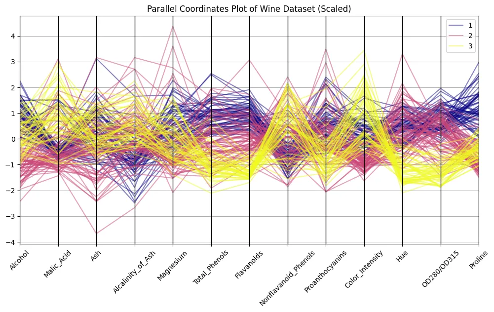

Bear in mind the image from above? The distinction is hanging, eh? Now we are able to discern patterns. Attempt to distinguish clusters of strains related to every wine class to search out out what options are most distinguishable.

Function Choice

Did you uncover one thing? Appropriate! I acquired the impression that alcohol, flavonoids, color depth, and proline present nearly textbook-style patterns. Let’s filter for these and attempt to see if a curation of options helps make our observations much more hanging.

chosen = ["Alcohol", "Flavanoids", "Color_Intensity", "Proline", "Class"] plt.determine(figsize=(10,6)) parallel_coordinates(scaled_df[selected], 'Class', colormap='coolwarm', alpha=0.6) plt.title("Parallel Coordinates Plot of Chosen Options") plt.xticks(rotation=45) plt.present()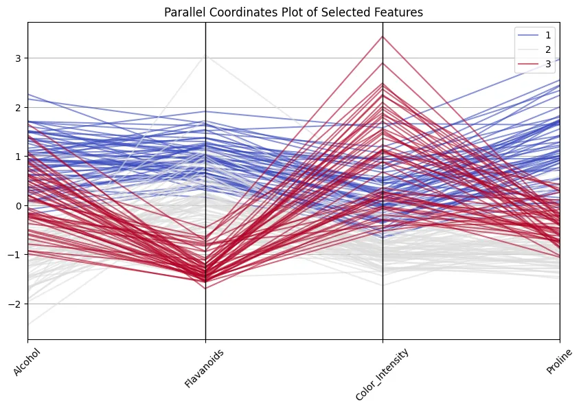

Good to see how class 1 wines all the time rating excessive on flavonoids and proline, whereas class 3 wines are decrease on these however excessive in color depth! And don’t assume that’s a useless train… 13 dimensions are nonetheless alright to deal with and to examine, however I’ve encountered instances with 100+ dimensions, making lowering dimensions crucial.

Including Interplay

I admit: the examples above are fairly mechanistic. When writing the article, I additionally positioned hue subsequent to alcohol, which made my properly proven lessons collapse; so I moved color depth subsequent to flavonoids, and that helped. However my goal right here was to not provide the good copy-paste piece of code; it was fairly to indicate you the usage of parallel coordinates based mostly on some easy examples. In actual life, I might arrange a extra explorative frontend. Plotly parallel coordinates, as an illustration, include a “brushing” function: there you possibly can choose a subsection of an axis and all polylines falling inside that subset will probably be highlighted.

You can even reorder axes by easy drag and drop, which regularly helps reveal correlations that have been hidden within the default order. Trace: Strive adjoining axes that you just suspect to co-vary.

And even higher: scaling isn’t essential for inspecting the info with plotly: the axes are routinely scaled to the min- and max values of every dimension.

Right here’s a code so that you can reproduce in your Colab:

import plotly.specific as px # Hold class as a separate column; Plotly's parcoords expects numeric color for 'colour' df["Class"] = df["Class"].astype(int) fig_all = px.parallel_coordinates(     df,     colour="Class",                  # numeric color mapping (1..3)     dimensions=options.columns,         labels={c: c.exchange("_", " ") for c in scaled_df.columns}, ) fig_all.update_layout(     title="Interactive Parallel Coordinates — All 13 Options" ) # The file beneath could be opened in any browser or embedded by way of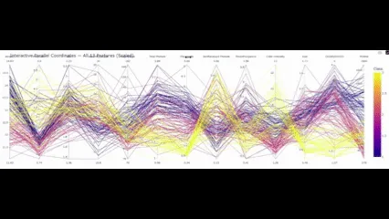 

So with this closing ingredient in place, what conclusions will we draw?

Conclusion

Parallel coordinates usually are not a lot in regards to the exhausting numbers, however rather more in regards to the patterns that emerge from these numbers. Within the Wine dataset, you can observe a number of such patterns – with out operating correlations, doing PCA, or scatter matrices. Flavonoids strongly assist distinguish class 1 from the others. Color depth and hue separate lessons 2 and three. Proline additional reinforces that. What follows from there’s not solely that you may visually separate these lessons, but additionally that it offers you an intuitive understanding of what separates cultivars in apply. 

And that is precisely the power over t-SNE, PCA, and many others., these methods challenge knowledge into elements which can be wonderful in distinguishing the lessons… However good luck attempting to elucidate to a chemist what “element one” means to him. 

Don’t get me mistaken: parallel coordinates usually are not the Swiss military knife of EDA. You want stakeholders with an excellent grasp of information to have the ability to use parallel coordinates to speak with them (else proceed utilizing boxplots and bar charts!). However for you (and me) as a knowledge scientist, parallel coordinates are the microscope you could have all the time been eager for.

Continuously Requested Questions

Because the CDAO at Fischer, I’m a seasoned skilled with over 15 years of expertise within the area of information science. With a Ph.D. in economics and 5 years of expertise as an Assistant Professor for Financial Principle, I’ve developed a deep understanding of social norm compliance and its impression on decision-making.
I’m additionally a famend convention speaker and podcast participant, sharing my experience on a variety of matters associated to knowledge science and enterprise technique. My background contains working as an A.I. Evangelist for STAR Cooperation and in technique and administration consulting with a deal with after-sales pricing. This expertise has allowed me to develop a broad ability set that features knowledge science, product administration, and technique growth.
Earlier than my present job, I used to be accountable for managing a big Knowledge Science Heart of Excellence at E. Breuninger, the place I led a group of information scientists and product managers. I’m enthusiastic about leveraging knowledge to drive enterprise choices and obtain tangible outcomes, and I’ve a confirmed observe document of success on this space.
With a deep data of economics, psychology, and knowledge science, I’m wanting ahead to skilled exchanges with any group trying to drive progress and innovation by means of data-driven insights.